

Tomography
How it works - theory
In section tomography, the data obtained is in the form of sections which cut through the specimen (see tomography). In the case of OCT these sections are 1-dimensional lines which cut through the specimen parallel to the optical axis (the z-axis). The specimen is effectively "sampled" at points along this 1D section. The positions of these sample points along the z-axis is calculated from the time taken for reflected photons to arrive back at the objective lens. In the case of confocal microscopy the sections are effectively zero-dimensional single points in space. In this case the position of the point along the z-axis is known because it lies exactly on the focal plane of the objective lens (see confocal microscopy).
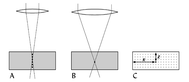
Diagram illustrating the principle of section tomography. (A) OCT scans one line at a time. Distances along the line are determined by calculating how long it takes for light to travel down through the specimen and back up again from that point. (B) Confocal microscopy effectively samples the specimen at a single point. (C) Every sampled point in these techniques has a specified coordinate in 3-D space. By sampling an array of points through the entire volume (grey dots), a complete 3-D description of the specimen is built-up.
In projection tomography, the data obtained from the specimen does not have a direct mapping to a single position in 3-D space. Instead, each piece of data indicates the total amount of light absorbed or emitted along a straight line through the specimen.
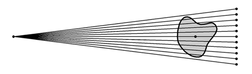
A typical projection tomography set-up, such as a medical X-ray CT scanner. Rays are emitted from the source (dot on the left), and progress in straight lines through the specimen (grey shape) to the ray detectors (line of dots on the right). No focusing, refracting or scattering of rays occurs.
The data collected acts essentially like a shadow of the object. Where the object is thicker the shadow is darker. This data does not map to a specific position within the object, but when added to similar data collected from other angles, it contributes to a full description of the object (see tomography). The algorithm which performs this calculation is called a back-projection algorithm.
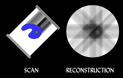
After a large number of projections have been collected during scanning, they are reconstructed into a representation of the original object using a back-projection algorithm.
In standard forms of projection tomography (such as those using X-rays, g-rays or electrons beams) those rays which are not absorbed pass straight through the specimen to the detector without any significant scattering or refraction. This is important for the reconstruction process, as the path of each ray must be accurately known. In optical projection tomography (OPT) this is not strictly possible. Light is scattered to a certain extent, and is certainly refracted as it passes through the necessary magnifying optics of the microscope. Nevertheless, we have shown that the resultant data, captured by a CCD digital camera on the microscope, is a close enough approximation to parallel projection data to generate good quality reconstructions.
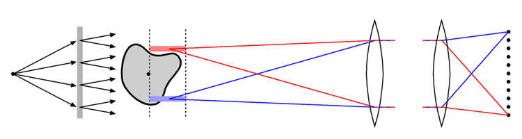
The optical projection tomography set-up. Light from a lamp (black dot on the left) is converted into an even illumination by the diffuser (vertical grey bar). It then passes through the specimen (grey shape) abd is focused by the optics of the microscope onto a CCD imaging chip (row of black dots). Although light rays do not follow straight paths through the specimen, the intensity recorded at each position on the camera chip approximates a projection through the focused part of the specimen (region between dashed lines).
The back-projection algorithm adds projections to the reconstruction successively, gradually building-up the final image. The following movie (click on image) demonstrates this accumulation, for a section through an E10.5 mouse embryo (see Studies: MAP TS19).